Key idea of iterative methods for eigenvalue computation

Remember one of the steps in computing eigenvalues

$$Q^{T}AQ=H$$

This was the step where $A$ is transformed to an upper Hessenberg matrix to reduce the computational cost of the QR iteration algorithm.

Let’s rewrite the equality as

$$AQ=QH$$

where $H$ is upper Hessenberg.

Upon inspection, once $q_1$ is chosen, the other vectors in $Q$ are fixed:

$$\begin{array}{c}(q_1,\dots ,q_j)\to q_{j+1}\\ A{q}_j=\sum _{k=1}^{j+1}{h}_{kj}{q}_k\end{array}$$

This algorithm is very similar to the Gram-Schmidt algorithm for the QR factorization but it uses $A{q}_j$.

We get column $j$ of $h$

$$h_{kj}=q_k^{T}A{q}_j,k\le j$$

Let’s project $A{q}_j$ on $q_k$:

$$h_{j+1,j}{q}_{j+1}=A{q}_j-\sum _{k=1}^j{h}_{kj}{q}_k$$

$h_{j+1,j}$ is the norm of the right-hand-side vector; once we have $h_{j+1,j}$, we get:

$$q_{j+1}=h_{j+1,j}^{-1}(A{q}_j-\sum _{k=1}^j{h}_{kj}{q}_k)$$

Iteration §

Start from $q_1$. Then:

1. Compute $A{q}_j$. This requires a sparse matrix-vector product.
2. $h_{kj}=q_k^{T}A{q}_j$, $1\le k\le j$.
3. $h_{j+1,j}{q}_{j+1}=A{q}_j-{\sum }_{k=1}^j{h}_{kj}{q}_k$

• If you continue this iterative process to the end, you get a dense matrix $H$.
• The sparsity advantage is lost.
• But what happens if we stop before the end?
• By using the top left $k\times k$ block of $H$ we will be able to approximately compute eigenvalues and solve linear systems. As long as $k$ remains small, this can be computationally very fast.

Details of the iterative process §

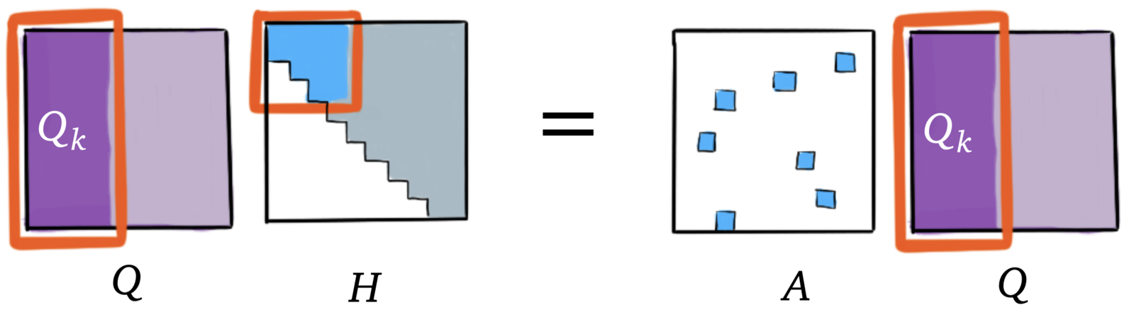
If we stop at step $k$, we get the following equation:

$$Q_k{H}_k+h_{k+1,k}{q}_{k+1}{e}_k^T=A{Q}_k$$

and

$$Q_k{H}_k\approx A{Q}_k$$

if $h_{k+1,k}$ is small. This suggests using the following matrix $H_k$

$$H_k=Q_k^{T}A{Q}_k$$

instead of $A$.

From that point, iterative algorithms replace a calculation using $A$ with a calculation using $H_k$. $H_k$ is a small matrix, and “direct” methods are efficient and fast.

The main application cases are the conjugate gradients method (which we will cover later) and the Arnoldi process.